Electricity Consumption Forecasting in Algeria: A Comparison of ARIMA and GM (1,1) Models

Abstract

  The pivotal role of electrical energy in propelling a nation's economic development cannot be overstated. A deficiency in the efficient consumption of electricity not only acts as a hindrance to economic growth but also constitutes a potential threat to national security. Recognizing the gravity of this relationship, scholars and policymakers have directed substantial attention towards the exploration of electricity consumption patterns and the development of predictive models. Consequently, a diverse array of models and methodologies has been employed to forecast electrical energy consumption.
  Within this context, the present research delves into a comparative analysis of two prominent forecasting methods,  ARIMA and GM (1,1) grey modeling techniques, with a specific focus on predicting electricity consumption in Algeria. The assessment of these models' performances was conducted using the average percentage of absolute MAPE, employing annual data collected from Algeria spanning the extensive period from 1982 to 2020. 
  The research findings underscore the paramount importance of accurate forecasting in this domain. Notably, the ARIMA model (1,1,0) emerged as the frontrunner, exhibiting superior predictive capabilities when juxtaposed with the GM (1,1) model, as evidenced by the MAPE standard. This nuanced examination contributes to the scholarly discourse on electricity consumption prediction, offering insights that can inform strategic decision-making and policy formulation in the pursuit of sustainable and secure energy practices.

Keywords: Forecasting, Electricity Consumption, Autoregressive Integrated Moving Average (ARIMA) Model, Grey modelling (1,1)

1. Introduction

Electrical energy is one of the main pillars in the economic development of countries, as any lack of consumption of this energy may lead to a slowdown in economic development and economic growth and may even threaten national security (Panklib et al., 2015). [1] Therefore, electricity consumption has become a topic of great importance because of the increasing demand for energy worldwide, mainly fueled by growing economic activities (Kandananond, 2011). [2] Given this fact, a sound forecasting technique is essential for accurate investment planning of energy production, generation, and distribution (Bianco et al., 2010). [3]

In recent decades, many methods in the literature for forecasting used different techniques for electricity consumption prediction. The most common models for this purpose are the autoregressive integrated moving average, artificial neural networks (ANN), support vector regression (SVR), hybrid models, and fuzzy logic methods.

Algeria has recently worked to develop the state in all fields, whether economic, social, political, etc.

As the Electric energy index indicates a factor for the development of any country, the government of Algeria should monitor electricity consumption growth; forecasting is essential for the practical application of energy. Accurate forecasts of electricity consumption are vital when demand is growing faster. On the other hand, the values of electricity consumption in Algeria can be viewed as volatile and increasing.

The present paper aims to analyze and forecast electricity consumption in Algeria utilizing The grey forecasting GM (1,1) model, invented by Deng, 1982 (Wang et al., 2018) [4], which has been regarded as one of most widely utilized prediction approaches because its requirement of few samples and high forecasting accuracy, and autoregressive integrated moving average(ARIMA).

The rest of the paper is organized as follows. In Section 2, some related works are introduced. Section 3 describes the methodology. Section 4 presents the main results and discussion. Finally, the conclusions and future works are presented in Section 5.

1. Literature Review

Electricity consumption forecasting has received prominent attention among researchers today using different models (Oğcu et al., 2012). [5] This study employed seasonal SVR and ANN models to develop the best model for predicting electricity output between 2010 and 2011. The study’s results provided empirical evidence that electricity consumption in Turkey will increase soon. (Rathnayaka, et al 2014). [6] GM (1, 1) and Grey Model (1, 1) have been used for forecasting results. The performance of the proposed technique has been compared with the existing Auto-regressive moving average forecasting model. Annual power generation and forecasting data in Sri Lanka were used. MAPE, MSD and MSE accuracy testing results show that GM (1, 1) outperformed compared to model fitting and forecasting. (Hussain et al, 2016). [7] This paper applies Holt-Winter and Autoregressive Integrated Moving Average (ARIMA) models on time series secondary data from 1980 to 2011 to forecast total and component-wise electricity consumption in Pakistan. Results reveal that Holt-Winter is the appropriate model for forecasting electricity consumption in Pakistan. (ŞİŞMAN, 2017), [8] proposition of a new approach by comparing grey prediction and ARIMA models with the Model of Analysis of the Energy Demand in Turkey from 1970 until 2013. Results have revealed that ARIMA and GP give better results than MAED to forecast long-term perspectives. In addition, it appears that the original ARIMA and GM (1,1) models have powerful forecasting models. (Amber et al., 2018). [9] This paper uses Multiple Regression (MR), Genetic Programming (GP), Artificial Neural Networks (ANN), Deep Neural Networks (DNN) and Support Vector Machine (SVM) to forecast the electricity consumption of an administration building located in London, United Kingdom. Results demonstrate that ANN performs better than all other four techniques. (Jain et al., 2018). [10] In this paper, an attempt is made to forecast electricity consumption using the ARIMA model. The mean absolute percentage error (MAPE) measures forecast accuracy. Results show that the ARIMA model has the potential to compete with existing techniques for electricity consumption forecast. (Leite et al., 2022). [11] This paper aimed to apply time-series forecasting models (the Holt–Winters, SARIMA, Dynamic Linear Model, and TBATS (Trigonometric Box–Cox transform, ARMA errors, Trend, and Seasonal components and NNAR (neural network autoregression) and MLP (multilayer perceptron). The results indicate that the MLP model obtained the best forecasting performance for the electricity consumption of the Brazilian industry under analysis. (Bilgili et al, 2022). [12] In this study, four time-series methods: long short-term memory (LSTM) neural network, adaptive neuro-fuzzy inference system (ANFIS) with subtractive clustering (SC), ANFIS with fuzzy means (FCM), and ANFIS with grid partition (GP) were implemented for forecasting electricity consumption. Results reveal the LSTM model generally outperformed all ANFIS models.

1. Methodology

3.1. The ARIMA Model

The model was proposed by Box-Jenkins in 1970, as it consists of autoregressive models, which are denoted by (AR) of order (p), and moving average models, which are denoted by (MA) of order (q), and (d) indicates the number of times the time series differences should be taken to make it stable (In most cases d = 1) (Fattah et al., 2018). [13]

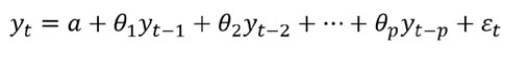
• TheAutoregressive (AR) Model

The equation below takes the following: (Goshit, &Iorember, 2018) [14]

• • TheMovingAverage (MA) Model

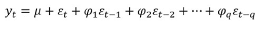
 can also be designed as follows:

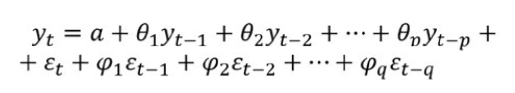
• TheAutoregressiveIntegratedMovingAverage (ARIMA)

The formula for ARIMA could be represented as: (Grigonytė&Butkevičiūtė, 2016) [15]

Developing the ARIMA model requires to follow four basic steps: identification, estimation, diagnostic checking, and forecasting (Bari et al., 2015) [16]

differencing to achieve stationary Stability analysis of the time series is necessary for the modelling process. We consider a series stable if its arithmetic average, variance, and covariance over time are constant (ATIL& MAHFOUD, 2021). [17] We can find out, however, that the series is unstable by The autocorrelation functions (ACF) or partial autocorrelation functions (PACF) (Udom&Phumchusri, 2014) [18], or Augmented Dicky-Fuller Test’s (ADF) and PP Test’s.

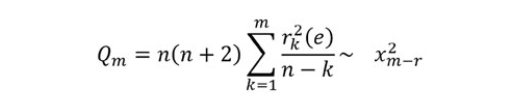
Step one is to identify (p, q), which the orders of the AR model and MA model and is the most important, using the autocorrelation (ACF) and partial autocorrelation (PACF) functions are taken to identify the models because they show different features of the functions (Guha&Bandyopadhyay 2016). [19] For AR (p), the ACF tails off at the order of p but PACF cutoff; for MA (q), the ACF cutoff but PACF tails off at the order of q; for ARMA (p, q), none of the ACF and PACF tail off, and to select as the best suitable model for forecasting (Mondal et al, 2014) [20], using BIC (Bayesian Information Criterion) and AIC (Akaike Information Criterion) values. Step two is Estimating the coefficients of the formulation using the Maximum Likelihood method (Eissa, 2020). [21] Step three is the Checking of the Model, where the model must be checked for adequacy by considering the properties of the residuals and whether the residuals from an ARIMA model must have a normal distribution and should be random. An overall check of model adequacy is provided by the Ljung-Box Q statistic (Kumar&Anand, 2014). [22] The test statistic Q is:

and step fourth is Forecasting; once the three previous steps of the ARIMA model is over, we can obtain forecasted values by estimating the appropriate model free from problems (Padhan, P. C. 2012). [23]

• GM (1,1) Model

The meaning of the grey system theory (GST), proposed by Deng Julong in 1982 (Ikram et al., 2019) [24], goes back to the origin of the color grey, which is a mixture of white and black. Where black indicates a complete lack of information, while white indicates complete information,. In other words, this theory refers to dealing with the lack of information, that is, dealing with small and weak data (Wu et al. 2015). [25] In addition, it only needs four recent data points and tries to process them through the process of grey generation to achieve reliable and acceptable accuracy for future prediction (Hu 2017). [26]

It has become one of the essential methods that can be applied to forecast and modelling in economic, social, and science fields (Zhou& Ma, 2020). [27]

The (GST) is based on the GM (1,1) grey model of the first order (i.e. differential equations of the first order), where the solution of the differential equation is solved with the least square method, with one variable (Lin et al. 2011). [28]

The steps in the construction of the grey forecasting model GM (1,1) are as follows (Tsai et al. 2017) [29], (Yuan et al 2016) [30]:

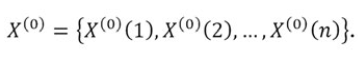
• • Define all of the past data obtained as the original series:

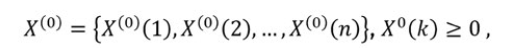
 , , Where  is the non-negative original time sequence (Wang el al 2018) [31], and k = 1, 2,..n .

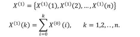
• • Perform one primary accumulation generating operation sequence (AGO) to add together the established original series and obtain the following generated series:

• • The GM (1, 1) model can be built by establishing a first-order differential equation with one variable , as follows:

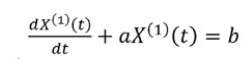
 , where the parameters is called the development coefficient and is called grey input and is a constant term (Yang el al 2021). [32]

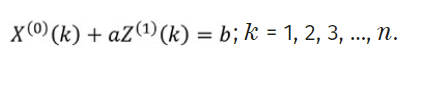
• The discrete from of the GM (1, 1) differential equation model is expressed as follows:

           ;

Where 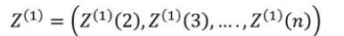 and is said to be mean series of

• • In order to obtain the parameters A and B, Used the least square method and differential and difference equations, that is:

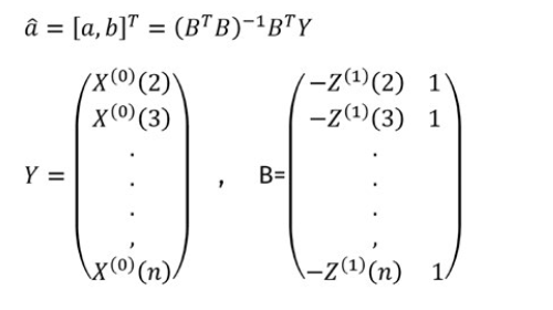
    ,     B=

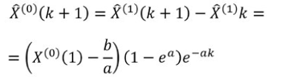
• • we can derive the estimated first-order AGO sequenceand the estimated inversed AGO sequence , using the least squares estimation, and is also called the time response function, and it is as follows (chiou et al. 2004)[33]:

   ,

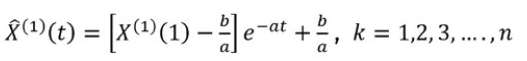
• • And then, the equation of time response sequence is depicted in the following equation:

   ,

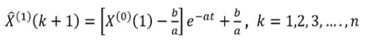
Finally, forecasting equation is generated, and the fitted values and predicted values of the sequence X can be calculated.

1. Empirical Results and Discussion

The data used in this study is the annual electricity consumption in Algeria. Intended yearly data were obtained from https://countryeconomy.com/energy-and-environment/electricity-consumption/algeria, from 1980 to 2021, as presented in Figure 1. The dataset consists of a total of 42 observations. The data set was split from January 1980 to 2015 for training purposes, whereas the remaining was used for testing purposes from 2016 to 2021 for both methods (ARIMA and GM (1,1)).

Figure 1. Time series plot of electricity consumption in Algeria

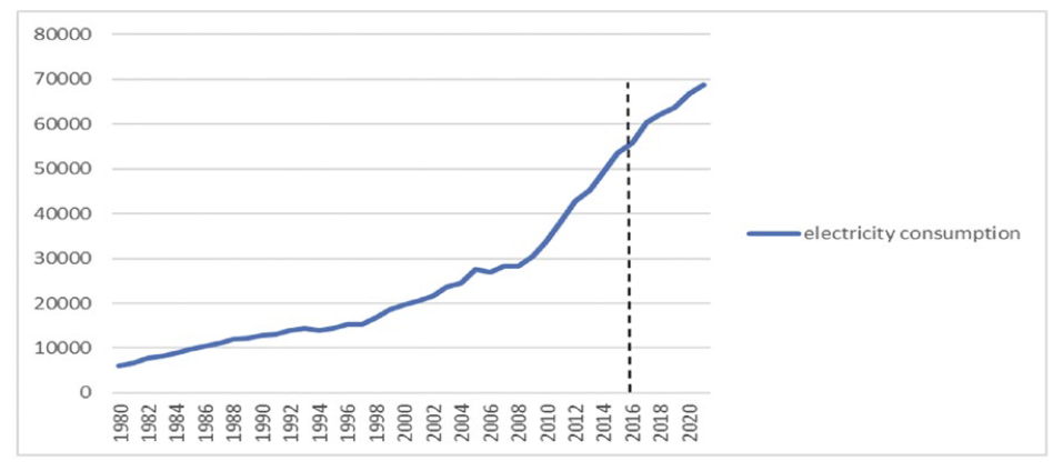
Source: Author’s calculations using Eviews12

In Figure 1, the time series plot of electricity consumption in Algeria shows it had been increasing from the starting point to 2006 to 2008. There was a slowdown in electricity consumption, but again, it increased sharply. This is due to several reasons, including population growth on the one hand, given that the most significant consumption tends to the residential sector, especially in recent years, as the state paid attention to infrastructure and work to attract foreign investment and promote the industrial to obtain sustainable development.

Table 1: Results of Descriptive Statistics

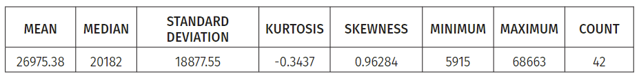
Source: Author’s calculations using Eviews12

We note through the above table that the minimum value was 5915, and the maximum value was 68663; the mean value was positive (26975.38), the median value was 20182, and the standard deviation value was 18877.55. The Electricity consumption value was positively skewed (0.96284). The kurtosis value for electricity consumption is at -0.3437. And the count of observations was 42.

4.1. The ARIMA Model

To verify the stability, we use the Augmented Dicky-Fuller Test (ADF) stability test and the Phillip-perron Tests (PP). The results of the ADF and PP tests are reported in Table 2.

The variable of electricity consumption is non-stationary. The electricity consumption series must be differentiated once to be stationary; hence, the order of integration d equals 1.

Table 2: Augmented Dickey Fuller Unit Root and phillip-perron Tests

Notes: * indicates statistical significance at the 1% significance level, ** indicates statistical significance at the 5% significance

Source: Author’s calculations using Eviews12

Figure 2: Autocorrelation and Partial Autocorrelation function.

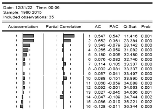
Source: Author’s calculations using Eviews12

Figure 2 below represents the plot of the correlogram (autocorrelation function, ACF) and Autocorrelations (ACF) of the first differenced series by lag for lags 1 to 16 of the time series of the Electricity consumption in Algeria.

After the experiment, we will select the most suitable model for forecasting out of the proposed models, with the lowest BIC (Bayesian Information Criterion) and AIC (Akaike Information Criterion) values. The results indicated that the most appropriate ARIMA model to forecast was ARIMA (1,1,0).

Table 3: Model Estimation

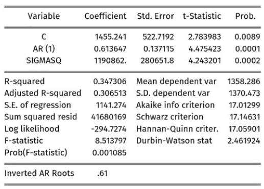
Source: Author’s calculations using Eviews12

4.2. Building and Application the GM (1,1) Model of Electricity Consumption in Algeria:

Data of electricity consumption in Algeria for the past 1980-2015 years were selected as the training set, to construct to establish the original time series .

After that, we calculated the primary accumulation sequence, to reduce the randomness of time series.

Following, we will GM (1,1) model was established via X1, and to estimate parameters, we use the method of least squares. According to data of the electricity consumption, we obtain:

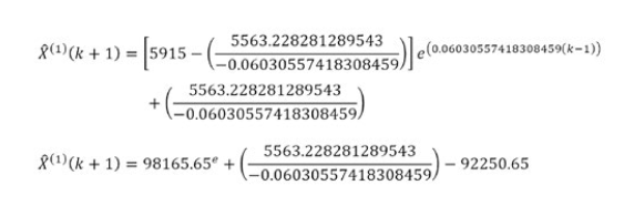
a= -0.06030557418308459b=5563.228281289543 

After obtaining the values of (a) and (b), they are introduced into the differential model corresponding to the GM (1,1) model, and the response function could be solved, to obtain the GM (1,1) prediction model, as follows:

Finally, the back difference ratio can be calculated, which is:

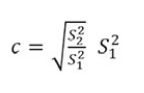
Where:

C is the index of the accuracy of the reaction model.

 is the variance of the original data:=

 is the residual al variance:

Knowing that the smaller the c, the higher the accuracy of the model.

and after testing, C = = 0.13720447115478135.

According to Table 4, which represents accuracy grade reference table.

C value , GM (1,1) The prediction accuracy level is: OK or Good.

Table 4: Accuracy Grade Reference Table

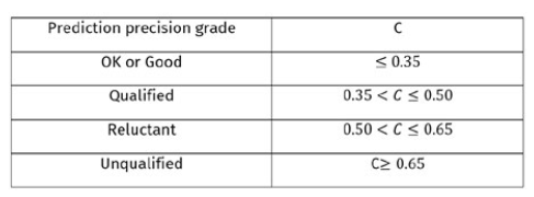
Source : Zhao, M., Zhao, D., Jiang, Z., Cui, D., Li, J., &Shi, X. (2015). [34] The gray prediction GM (1, 1) model in traffic forecast application. Mathematical modelling of engineering problems, 2(1), 17-22

Therefore, the GM (1,1) model could be used to test the Electricity consumption of Algeria.

The comparison of the predictive accuracy for the above two forecasting models of testing sample data is presented in Table 5. The mean absolute percentage error (MAPE) is utilized, which measures the predicting accuracy of the model using a statistical method as defined in Table 1.

Table 5: Forecasting Values and Performance Evaluation of Actual Values, GM (1,1), ARIMA (1,1,0) for Set Testing Sample Data.

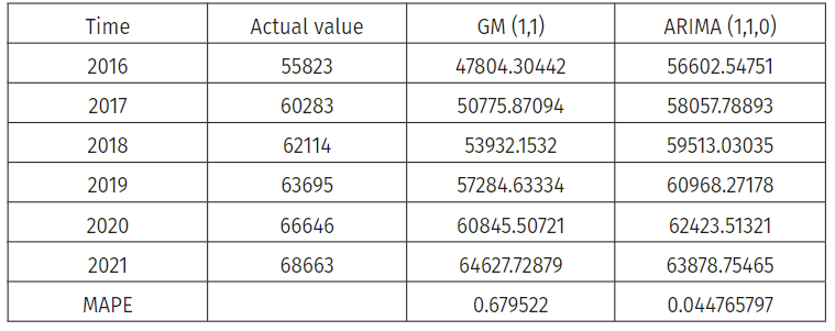
Source: Prepared by researchers

The table above explains that the ARIMA (1,1,0) model forecasting is better than GM (1,1) based on the mean absolute percentage error (MAPE). The MAPE value of testing sample data (2016-2021) for GM (1,1) and ARIMA (1,1,0) is 0.679522 and 0.044765797, respectively. ARIMA (1,1,0) has higher forecast accuracy than other forecasting models.

Figure 2: Curves for the models ARIMA (1,1,0) and GM (1,1).

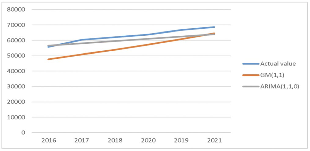
Source: Prepared by researchers

Figure 2 shows the width of the curves for the ARIMA (1,1,0) and GM (1,1) models. The forecasting results point out that the values predicted by the ARIMA model are very close to the original values of Algeria’s electricity consumption from 2016 to 2020 compared to the GM model.

Using the ARIMA (1,1,0) model, the annual electricity consumption was forecasted until 2030.

The forecasting values of electricity demand are given in Table 6.

Table 6: Forecasting Value of the ARIMA Model.

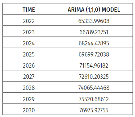
Source: Prepared by researchers

As revealed by the prediction results forecasted by the ARIMA (1,1,0) model, based on 2022, electricity consumption will continue to increase annually for the next nine years.

1. Conclusions

This study aims to provide energy policymakers and planners with a guideline for choosing the most appropriate forecasting techniques to forecast electricity consumption trends in Algeria accurately. This paper’s main objective is to forecast Algeria’s annual electricity consumption for the 1980-2021 period. Based on GM (1,1) and Autoregressive Integrated Moving Average (ARIMA) to select the most appropriate fit. The results show that the ARIMA (1,1,0) model exhibits good forecasting ability according to the MAPE criteria, Compared with Model GM (1,1).

The Algerian state might use the study’s outcome to develop energy policies and measures on energy conservation and alternative energy.

In the future, the following works may focus on forecasting electricity consumption using RBF Artificial Neural Networks, Hybrid Model GM (1,1)-ARCH, and Hybrid ARIMA-GM (1,1).

References

1. Panklib, K., Prakasvudhisarn, C., &Khummongkol, D. (2015). Electricity consumption forecasting in Thailand using an artificial neural network and multiple linear regression. Energy Sources, Part B: Economics, Planning, and Policy, 10(4), 427-434.
2. Kandananond, K. (2011). Forecasting electricity demand in Thailand with an artificial neural network approach. Energies, 4(8), 1246-1257.
3. Bianco, V., Manca, O., Nardini, S., &Minea, A. A. (2010). Analysis and forecasting of nonresidential electricity consumption in Romania. Applied Energy, 87(11), 3584-3590.
4. Wang, Z. X., Li, Q., & Pei, L. L. (2018). A seasonal GM (1, 1) model for forecasting the electricity consumption of the primary economic sectors. Energy, 154, 522-534.
5. Oğcu, G., Demirel, O. F., &Zaim, S. (2012). Forecasting electricity consumption with neural networks and support vector regression. Procedia-Social and Behavioral Sciences, 58, 1576-1585.
6. Rathnayaka, R. M. K. T., &Seneviratne, D. M. K. N. (2014). GM (1, 1) analysis and forecasting for efficient energy production and consumption. International Journal of Business, Economics and Management Works, 1(1), 6-11.
7. Hussain, A., Rahman, M., &Memon, J. A. (2016). Forecasting electricity consumption in Pakistan: The way forward. Energy Policy, 90, 73-80.
8. ŞİŞMAN, B. (2017). A comparison of ARIMA and grey models for electricity consumption demand forecasting: The case of Turkey. KastamonuÜniversitesiİktisadiveİdariBilimlerFakültesiDergisi, 13(3), 234-245.
9. Amber, K. P., Ahmad, R., Aslam, M. W., Kousar, A., Usman, M., & Khan, M. S. (2018). Intelligent techniques for forecasting electricity consumption of buildings. Energy, 157, 886-893.
10. Jain, P. K., Quamer, W., &Pamula, R. (2018, April). Electricity consumption forecasting using time series analysis. In International Conference on Advances in Computing and Data Sciences(pp. 327-335). Springer, Singapore.
11. Leite Coelho da Silva, F., da Costa, K., Canas Rodrigues, P., Salas, R., &López-Gonzales, J. L. (2022). Statistical and Artificial Neural Networks Models for Electricity Consumption Forecasting in the Brazilian Industrial Sector. Energies, 15(2), 588.
12. Bilgili, M., Arslan, N., ŞEKERTEKİN, A., & YAŞAR, A. (2022). Application of long short-term memory (LSTM) neural network based on deeplearning for electricity energy consumption forecasting. Turkish Journal of Electrical Engineering and Computer Sciences, 30(1), 140-157.
13. Fattah, J., Ezzine, L., Aman, Z., El Moussami, H., &Lachhab, A. (2018). Forecasting of demand using ARIMA model. International Journal of Engineering Business Management, 10, 1847979018808673.
14. Goshit, G. G., &Iorember, P. T. SHORT-TERM INFLATION RATE FORECASTING IN NIGERIA: AN AUTOREGRESSIVE INTEGRATED MOVING AVERAGE (ARIMA) AND ARTIFICIAL NEURAL NETWORK (ANN) MODELS.
15. Grigonytė, E., &Butkevičiūtė, E. (2016). Short-term wind speed forecasting using ARIMA model. Energetika, 62(1-2).
16. Bari, S. H., Rahman, M. T., Hussain, M. M., & Ray, S. (2015). Forecasting monthly precipitation in Sylhet city using ARIMA model. Civil and Environmental Research, 7(1), 69-77.
17. ATIL, A., & MAHFOUD, B. (2021). Evolution of Crude Oil Prices during the COVID-19 Pandemic: Application of Time Series ARIMA Forecasting Model. Delta University Scientific Journal, 4(1), 1-12.
18. Udom, P., &Phumchusri, N. (2014). A comparison study between time series model and ARIMA model for sales forecasting of distributor in plastic industry. IOSR Journal of Engineering, 4(2), 32-38.
19. Guha, B., &Bandyopadhyay, G. (2016). Gold price forecasting using ARIMA model. Journal of Advanced Management Science, 4(2).
20. Mondal, P., Shit, L., &Goswami, S. (2014). Study of effectiveness of time series modeling (ARIMA) in forecasting stock prices. International Journal of Computer Science, Engineering and Applications, 4(2), 13.
21. Eissa, N. (2020). Forecasting the GDP per Capita for Egypt and Saudi Arabia Using ARIMA Models. Research in World Economy, 11(1), 247-258.
22. Kumar, M., &Anand, M. (2014). An application of time series ARIMA forecasting model for predicting sugarcane production in India. Studies in Business and Economics, 9(1), 81-94.
23. Padhan, P. C. (2012). Application of ARIMA model for forecasting agricultural productivity in India. Journal of Agriculture and Social Sciences, 8(2), 50-56.
24. Ikram, M., Mahmoudi, A., Shah, S. Z. A., &Mohsin, M. (2019). Forecasting number of ISO 14001 certifications of selected countries: application of even GM (1, 1), DGM, and NDGM models. Environmental Science and Pollution Research, 26(12), 12505-12521.
25. Wu, L., Liu, S., Fang, Z., & Xu, H. (2015). Properties of the GM (1, 1) with fractional order accumulation. Applied Mathematics and Computation, 252, 287-293.
26. Hu, Y. C. (2017). Electricity consumption prediction using a neural-network-based grey forecasting approach. Journal of the Operational Research Society, 68(10), 1259-1264.
27. Zhou, F., & Ma, P. (2020). End-of-life Vehicle Amount Forecasting based on an Improved GM (1, 1) Model. Engineering Letters, 28(3).
28. Lin, C. S., Liou, F. M., & Huang, C. P. (2011). Grey forecasting model for CO2 emissions: A Taiwan study. Applied Energy, 88(11), 3816-3820.
29. Tsai, S. B., Xue, Y., Zhang, J., Chen, Q., Liu, Y., Zhou, J., & Dong, W. (2017). Models for forecasting growth trends in renewable energy. Renewable and Sustainable Energy Reviews, 77, 1169-1178.
30. Yuan, C., Liu, S., & Fang, Z. (2016). Comparison of China’s primary energy consumption forecasting by using ARIMA (the autoregressive integrated moving average) model and GM (1, 1) model. Energy, 100, 384-390.
31. Wang, Y. W., Shen, Z. Z., & Jiang, Y. (2018). Comparison of ARIMA and GM (1, 1) models for prediction of hepatitis B in China. PloS one, 13(9), e0201987.
32. Yang, F., Tang, X., Gan, Y., Zhang, X., Li, J., & Han, X. (2021). Forecast of freight volume in Xi’an based on gray GM (1, 1) model and Markov forecasting model. Journal of Mathematics, 2021.
33. Chiou, H. K., Tzeng, G. H., & Cheng, C. K. (2004). Grey prediction GM (1, 1) model for forecasting demand of planned spare parts in navy of Taiwan. In Proceedings World Automation Congress. Seville, Spain. Retrieved from https://ieeexplore. ieee. org/document/1439385
    
34. Zhao, M., Zhao, D., Jiang, Z., Cui, D., Li, J., &Shi, X. (2015). The gray prediction GM (1, 1) model in traffic forecast application. Mathematical modelling of  engineering problems, 2(1), 17-22